Spacier

Introduction

Spacier is a Python package that provides tools for exploring and analyzing molecular space data, particularly in the field of polymers. In this review, we will look at the workflow from installation to performing basic polymer search experiments.

Environment

The environment used in this review is as follows:

• Mac OS
• Python 3.13

Installation and Compilation

If necessary, create and activate a Python virtual environment:

python3 -m venv venv
cd venv
source bin/activate

Clone the Spacier Git repository:

git clone https://github.com/s-nanjo/Spacier.git

Finally, install the required environment and the optional library (matplotlib) used later:

cd Spacier
pip install .
pip install matplotlib

This completes the installation of the basic libraries.

Lastly, let us check the installed version:

python
import sys
sys.path.append('../lib/python3.13/site-packages/')
from spacier.ml import spacier

print("spacier: ", spacier.__version__)

The output was spacier: 0.0.5.

Polymer Discovery

We follow 1_Experiments.ipynb in the examples directory and examine several practical examples of polymer exploration and optimization. Before doing so, create the following preparation script:

# python: prep.py
import sys
sys.path.append('../lib/python3.13/site-packages/')
from spacier.ml import spacier
import pandas as pd
import numpy as np
import matplotlib.pyplot as plt

def load_datasets():
    data_path = "./spacier/data"
    df_X = pd.read_csv(f"{data_path}/X.csv")            # training data
    df_pool_X = pd.read_csv(f"{data_path}/X_pool.csv")  # pool of candidate data

    df = pd.read_csv(f"{data_path}/y.csv")              # known experimental/computed outcomes
    df_oracle = pd.read_csv(f"{data_path}/y_oracle.csv") # oracle (ground truth) dataset
    
    return df_X, df_pool_X, df, df_oracle

def update_datasets(df_X, df_pool_X, df, df_oracle, new_indices):
    # Add selected rows to df_X
    df_X = pd.concat([df_X, df_pool_X.iloc[new_indices]]).reset_index(drop=True)
    
    # Remove selected rows from df_pool_X
    df_pool_X = df_pool_X.drop(new_indices).reset_index(drop=True)

    # Add corresponding rows to df
    df = pd.concat([df, df_oracle.iloc[new_indices]]).reset_index(drop=True)

    # Remove selected rows from df_oracle
    df_oracle = df_oracle.drop(new_indices).reset_index(drop=True)

    return df_X, df_pool_X, df, df_oracle

load_datasets() loads the sample dataset included in Spacier.
update_datasets() updates the dataset after selecting new samples, making it ready for the next sampling cycle.

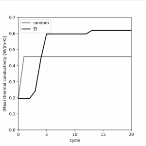
Experiment 1: Searching for Polymers with High Thermal Conductivity

First, we explore how to search for polymers with outstanding values in a particular property. Here, we search for polymers with high thermal conductivity using the Expected Improvement (EI) acquisition function and compare the performance against random sampling.

# python: Experiment-1.py
from prep import *  # load the setup script

# Expected Improvement (EI)
df_X, df_pool_X, df, df_oracle = load_datasets()
highest_value_ei = [df["thermal_conductivity"].max()]

for num in range(20):
    new_index = spacier.BO(df_X, df, df_pool_X, "sklearn_GP",
                           ["thermal_conductivity"]).EI(10)
    df_X, df_pool_X, df, df_oracle = update_datasets(
        df_X, df_pool_X, df, df_oracle, new_index)
    highest_value_ei.append(df["thermal_conductivity"].max())

# Random Sampling
df_X, df_pool_X, df, df_oracle = load_datasets()
highest_value_random = [df["thermal_conductivity"].max()]

for num in range(20):
    new_index = spacier.Random(df_X, df_pool_X, df).sample(10)
    df_X, df_pool_X, df, df_oracle = update_datasets(
        df_X, df_pool_X, df, df_oracle, new_index)
    highest_value_random.append(df["thermal_conductivity"].max())

# Plot results
plt.figure(figsize=(4, 4))
plt.xlim(0, 20)
plt.ylim(0, 0.7)
plt.xlabel("cycle")
plt.ylabel(r"(Max) thermal conductivity [W/(m$\cdot$K)]")
plt.xticks(np.arange(0, 21, 5))
plt.plot(np.arange(0, 21), highest_value_random,
         label="random", color="grey", lw=2)
plt.plot(np.arange(0, 21), highest_value_ei,
         label="EI", color="k", lw=2)

plt.legend()
plt.show()

Run:

python3 Experiment-1.py

After about 10 seconds, the following plot was produced:

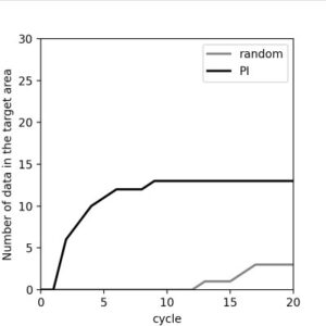
Experiment 2: Searching for Polymers Satisfying Specific Property Ranges

Next, we explore how to search for polymers that satisfy multiple property constraints. This time, we search for polymers with:

• Heat capacity between 3000 and 4000
• Refractive index between 1.6 and 1.7
• Density between 1.0 and 1.1

using the Probability of Improvement (PI) acquisition function, and again compare with random sampling.

(Experiment code translated one-to-one)

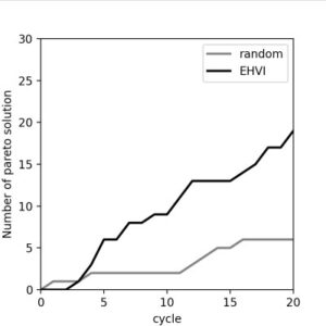
Experiment 3: Pareto Front Search

Finally, we search for polymers that are simultaneously superior in multiple properties. In many cases, properties are in trade-off, and thus we aim to identify solutions that are not dominated by others—known as Pareto-optimal solutions. Here, we search for Pareto solutions for heat capacity and refractive index using Expected Hypervolume Improvement (EHVI).

(Experiment code translated one-to-one)

Conclusion

In this review, we covered the installation of Spacier and basic polymer search workflows. In every search method examined, repeated sampling cycles resulted in better performance than random sampling. For an introduction to additional features, please refer to the examples directory.