Optuna

1. はじめに

Optunaは、ハイパーパラメータの最適化を効率的に行うためのPythonライブラリです。本記事ではHiggs Bosonに関する分類問題のデータセット（https://openml.org/search?type=data&sort=version&status=any&order=asc&exact_name=Higgs&id=45570）を使ったニューラルネットワークによる分類について、Optunaでハイパーパラメータの最適化を行います。本記事の内容はGoogle Colaboratoryで実行することを想定しています。

2. インストール

以下のコマンドを実行しインストールします。

!pip install optuna

3. 実行

まず、PyTorchでGPUを使うように設定します。

import torch
device = torch.device("cuda" if torch.cuda.is_available() else "cpu")
print(f"Using device: {device}")

次に、Higgsのデータセットの取得と前処理を行います。

from sklearn.datasets import fetch_openml
from sklearn.model_selection import train_test_split
from sklearn.preprocessing import StandardScaler

# データ取得
data = fetch_openml(name="Higgs", version=1)
X, y = data.data, data.target.astype(int)

# データの分割
X_train, X_test, y_train, y_test = train_test_split(X, y, test_size=0.2, random_state=42)

# 標準化
scaler = StandardScaler()
X_train = scaler.fit_transform(X_train)
X_test = scaler.transform(X_test)

# PyTorch Tensor に変換し GPU に転送
X_train_tensor = torch.tensor(X_train, dtype=torch.float32).to(device)
X_test_tensor = torch.tensor(X_test, dtype=torch.float32).to(device)
y_train_tensor = torch.tensor(y_train.values, dtype=torch.long).to(device)
y_test_tensor = torch.tensor(y_test.values, dtype=torch.long).to(device)

次に、PyTorchで隠れ層1のニューラルネットワークのモデルを定義します。ここで、ハイパーパラメータhidden_size(隠れ層のユニット数)を引数として与えます。

import torch.nn as nn
import torch.optim as optim

class DNN(nn.Module):
    def __init__(self, hidden_size):
        super(DNN, self).__init__()
        self.fc1 = nn.Linear(28, hidden_size)
        self.fc2 = nn.Linear(hidden_size, hidden_size)
        self.fc3 = nn.Linear(hidden_size, 2) 
    
    def forward(self, x):
        x = torch.relu(self.fc1(x))
        x = torch.relu(self.fc2(x))
        return self.fc3(x)

さらに、Optunaの最適化関数を定義します。hidden_size(隠れ層のユニット数)、lr(学習率)、batch_size(バッチサイズ)をハイパーパラメータとして学習を行い、テストデータで評価したaccuracy(精度)を返す関数として定義します。

import optuna

def objective(trial):
    # ハイパーパラメータの探索範囲
    hidden_size = trial.suggest_int('hidden_size', 32, 256)
    lr = trial.suggest_loguniform('lr', 1e-4, 1e-1)
    batch_size = trial.suggest_categorical('batch_size', [32, 64, 128])
    epochs = 20  # エポック数

    # モデルを GPU に配置
    model = DNN(hidden_size).to(device)
    criterion = nn.CrossEntropyLoss()
    optimizer = optim.Adam(model.parameters(), lr=lr)

    # DataLoader を作成
    train_dataset = torch.utils.data.TensorDataset(X_train_tensor, y_train_tensor)
    train_loader = torch.utils.data.DataLoader(train_dataset, batch_size=batch_size, shuffle=True)

    # 学習ループ
    for epoch in range(epochs):
        for X_batch, y_batch in train_loader:
            optimizer.zero_grad()
            outputs = model(X_batch)
            loss = criterion(outputs, y_batch)
            loss.backward()
            optimizer.step()

    # テストデータで精度を評価
    with torch.no_grad():
        y_pred = model(X_test_tensor)
        y_pred_classes = torch.argmax(y_pred, dim=1)
        accuracy = (y_pred_classes == y_test_tensor).sum().item() / len(y_test_tensor)

    return accuracy

最後に、Optunaでハイパーパラメータ最適化を実行します。デフォルトではTPESamplerというベイズ最適化を用いたサンプラーが使われます。

study = optuna.create_study(direction='maximize')  # 精度を最大化
study.optimize(objective, n_trials=30)  # 30回試行

# 最適なハイパーパラメータを表示
print("Best trial:")
print(f"  Accuracy: {study.best_value:.4f}")
print(f"  Params: {study.best_params}")

すると、23分ほどで最適化が終わり、以下のように最適なハイパーパラメータが表示されました。

Best trial:
  Accuracy: 0.7214
  Params: {'hidden_size': 50, 'lr': 0.0008382275385421477, 'batch_size': 64}

4. 結果の可視化

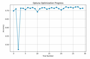
以下のコードで試行ごとの精度の変化をプロットすると、以下の図のようになりました。

import matplotlib.pyplot as plt
import pandas as pd

df = study.trials_dataframe()

plt.figure(figsize=(8, 5))
plt.plot(df["number"], df["value"], marker="o", linestyle="-")
plt.xlabel("Trial Number")
plt.ylabel("Accuracy")
plt.title("Optuna Optimization Progress")
plt.grid()
plt.show()

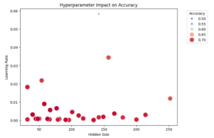
また、ハイパーパラメータと精度の関係を散布図で表すと以下のようになりました。最適なハイパーパラメータは左下の方にあることが分かります。なお、散布図が2次元のため、バッチサイズの情報が入っていないことに注意が必要です。

import seaborn as sns
import matplotlib.pyplot as plt

plt.figure(figsize=(8, 6))
scatter = sns.scatterplot(x=df["params_hidden_size"], y=df["params_lr"], size=df["value"], hue=df["value"], palette="coolwarm", sizes=(20, 200))

plt.legend(title="Accuracy", bbox_to_anchor=(1.05, 1), loc="upper left")

plt.xlabel("Hidden Size")
plt.ylabel("Learning Rate")
plt.title("Hyperparameter Impact on Accuracy")
plt.show()

5. おわりに

Optunaを使うと簡単にベイズ最適化を用いたハイパーパラメータの最適化をすることができました。今回は隠れ層が1層のニューラルネットワークを使いましたが、さらに精度を良くするためには隠れ層を増やすなどのモデルの改善が必要だと思われます。