Overview
ASE is a Python toolkit that standardizes the way researchers build, run, and analyze atomistic simulations. It defines a common Atoms object and Calculator interface so multiple electronic-structure and force‑field engines can be used through a consistent API. citeturn0search1turn1search2
What is ASE?
ASE is an open-source library centered on the Atoms data model for structure storage and manipulation. The Calculator abstraction unifies access to external codes (DFT, classical potentials, and ML potentials) and supports built-in workflows such as geometry optimization, molecular dynamics, and NEB. citeturn0search1turn0search5turn1search1
Key Features
- Unified calculator interface: run many simulation backends through the same Python API. citeturn0search1turn0search5
- Structure manipulation: create, transform, and analyze atomistic structures via the
Atomsobject. citeturn1search2turn0search1 - Built-in algorithms: optimizers, MD, NEB, and vibrational analysis are included in the core toolkit. citeturn0search5turn1search1
- Interoperability: ASE acts as glue between structure builders, DFT engines, and ML pipelines. citeturn0search1turn1search1
Installation
ASE is distributed via PyPI:
pip install ase
The official docs list the current release and installation guidance.
Example workflow (typical ASE pattern)
ASE workflows typically follow this pattern:
- Create an
Atomsobject (from a builder or file). - Attach a
Calculator(DFT, force field, or ML potential). - Run an optimizer or MD engine.
- Post‑process energies, forces, and trajectories.
This pattern is consistent across calculator backends and makes it easy to swap engines without changing downstream code.
Examples (materials informatics + computational materials)
I ran two local ASE examples to demonstrate both materials‑informatics‑style baselining and simulation‑workflow use.
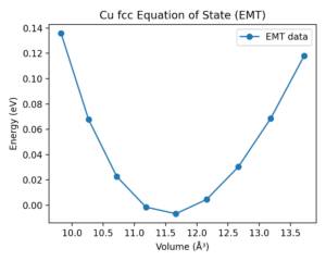
Example 1 · Bulk EOS baseline (materials informatics)
Goal: generate a structure‑energy baseline and fit an equation of state (EOS) for a cubic metal.
How ASE is used:
- Structure generation:
ase.build.bulk('Cu', 'fcc', a=a)creates an fcc Cu cell for each trial lattice constant. - Calculator binding:
atoms.calc = EMT()attaches a lightweight empirical calculator. - Energy/volume sweep: loop over
avalues, recordatoms.getpotentialenergy()andatoms.get_volume(). - EOS fit:
ase.eos.EquationOfState(volumes, energies).fit()returns equilibrium volume and bulk modulus. - Post‑processing: export CSV and parity plot for reporting.
Minimal implementation:
from ase.build import bulk
from ase.calculators.emt import EMT
from ase.eos import EquationOfState

a_values = [3.4, 3.45, 3.5, 3.55, 3.6, 3.65, 3.7, 3.75, 3.8]
energies, volumes = [], []
for a in a_values:
    atoms = bulk('Cu', 'fcc', a=a)
    atoms.calc = EMT()
    energies.append(atoms.get_potential_energy())
    volumes.append(atoms.get_volume())

eos = EquationOfState(volumes, energies)
v0, e0, B = eos.fit()
a0 = (4 * v0) ** (1.0 / 3.0)
Result (Cu fcc, EMT calculator):
- Best‑fit lattice constant
a0 = 3.590 Å - Bulk modulus
B = 0.832 eV/ų
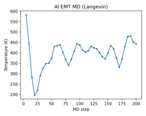
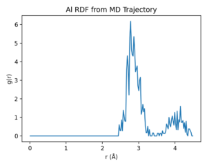
Example 2 · MD + RDF (computational materials)
Goal: run short molecular dynamics (MD) and analyze structure via the radial distribution function (RDF).
How ASE is used:
- Structure generation:
bulk('Al','fcc', a=4.05) * (4,4,4)builds a 4×4×4 supercell. - Calculator binding:
atoms.calc = EMT()provides forces/energies for MD. - Velocity initialization:
MaxwellBoltzmannDistribution(..., temperature_K=600)sets initial velocities. - MD integration:
Langevin(atoms, timestep, temperature_K=600, friction=0.02)runs 200 steps. - Trajectory + thermodynamics:
Trajectorycaptures frames;atoms.get_temperature()logs MD temperature. - RDF analysis:
ase.geometry.rdf.get_rdf(atoms, rmax=4.5, nbins=200)computes g(r) from the final structure.
Minimal implementation:
from ase.build import bulk
from ase.calculators.emt import EMT
from ase.md.langevin import Langevin
from ase.md.velocitydistribution import MaxwellBoltzmannDistribution
from ase import units
from ase.io import Trajectory
from ase.geometry.rdf import get_rdf

atoms = bulk('Al', 'fcc', a=4.05) * (4, 4, 4)
atoms.calc = EMT()
MaxwellBoltzmannDistribution(atoms, temperature_K=600)

dyn = Langevin(atoms, 2.0 * units.fs, temperature_K=600, friction=0.02)
traj = Trajectory('ase_md.traj', 'w', atoms)
dyn.attach(lambda: traj.write(atoms), interval=1)
dyn.run(200)

r, g_r = get_rdf(atoms, rmax=4.5, nbins=200)
Hands-on notes
- ASE is a thin but powerful orchestration layer; performance depends on the chosen calculator backend rather than ASE itself.
- ASE’s file I/O and
Atomsmodel make it easy to integrate with ML pipelines and dataset builders.
Conclusion
ASE is a foundational tool for computational materials workflows and a natural companion to Matminer and DScribe in MatDaCs reviews. It streamlines the path from structure creation to simulation and provides a stable API that keeps multi‑backend research scripts maintainable and reproducible.
References
- ASE documentation: https://ase-lib.org/ citeturn0search1
- ASE GitLab repository: https://gitlab.com/ase/ase citeturn1search0
- ASE paper: Hjorth Larsen et al., J. Phys.: Condens. Matter 29, 273002 (2017)