1. Introduction
Optuna is a Python library designed to efficiently perform hyperparameter optimization. In this article, we will use the Higgs Boson classification dataset (https://openml.org/search?type=data&sort=version&status=any&order=asc&exact_name=Higgs&id=45570) and apply Optuna to optimize the hyperparameters of a neural network classifier. This tutorial assumes that you are running the code on Google Colaboratory.
2. Installation
Run the following command to install Optuna:
!pip install optuna
3. Execution
First, set up PyTorch to use the GPU if available.
import torch
device = torch.device("cuda" if torch.cuda.is_available() else "cpu")
print(f"Using device: {device}")
Next, retrieve and preprocess the Higgs dataset.
from sklearn.datasets import fetch_openml
from sklearn.model_selection import train_test_split
from sklearn.preprocessing import StandardScaler

# Load dataset
data = fetch_openml(name="Higgs", version=1)
X, y = data.data, data.target.astype(int)

# Split data
X_train, X_test, y_train, y_test = train_test_split(X, y, test_size=0.2, random_state=42)

# Standardize
scaler = StandardScaler()
X_train = scaler.fit_transform(X_train)
X_test = scaler.transform(X_test)

# Convert to PyTorch tensors and move to GPU
X_train_tensor = torch.tensor(X_train, dtype=torch.float32).to(device)
X_test_tensor = torch.tensor(X_test, dtype=torch.float32).to(device)
y_train_tensor = torch.tensor(y_train.values, dtype=torch.long).to(device)
y_test_tensor = torch.tensor(y_test.values, dtype=torch.long).to(device)
Then, define a single-hidden-layer neural network in PyTorch. The hyperparameter hidden_size (the number of units in the hidden layer) is passed as an argument.
import torch.nn as nn
import torch.optim as optim

class DNN(nn.Module):
    def __init__(self, hidden_size):
        super(DNN, self).__init__()
        self.fc1 = nn.Linear(28, hidden_size)
        self.fc2 = nn.Linear(hidden_size, hidden_size)
        self.fc3 = nn.Linear(hidden_size, 2)

    def forward(self, x):
        x = torch.relu(self.fc1(x))
        x = torch.relu(self.fc2(x))
        return self.fc3(x)
Next, define the optimization function for Optuna. The hyperparameters hidden_size (hidden layer size), lr (learning rate), and batch_size are tuned. The function trains the model and returns the test accuracy.
import optuna

def objective(trial):
    # Define the search space
    hidden_size = trial.suggest_int('hidden_size', 32, 256)
    lr = trial.suggest_loguniform('lr', 1e-4, 1e-1)
    batch_size = trial.suggest_categorical('batch_size', [32, 64, 128])
    epochs = 20  # Number of epochs

    # Move model to GPU
    model = DNN(hidden_size).to(device)
    criterion = nn.CrossEntropyLoss()
    optimizer = optim.Adam(model.parameters(), lr=lr)

    # Create DataLoader
    train_dataset = torch.utils.data.TensorDataset(X_train_tensor, y_train_tensor)
    train_loader = torch.utils.data.DataLoader(train_dataset, batch_size=batch_size, shuffle=True)

    # Training loop
    for epoch in range(epochs):
        for X_batch, y_batch in train_loader:
            optimizer.zero_grad()
            outputs = model(X_batch)
            loss = criterion(outputs, y_batch)
            loss.backward()
            optimizer.step()

    # Evaluate on test data
    with torch.no_grad():
        y_pred = model(X_test_tensor)
        y_pred_classes = torch.argmax(y_pred, dim=1)
        accuracy = (y_pred_classes == y_test_tensor).sum().item() / len(y_test_tensor)

    return accuracy
Finally, run Optuna to optimize the hyperparameters. By default, the TPESampler (a Bayesian optimization-based sampler) is used.
study = optuna.create_study(direction='maximize')  # Maximize accuracy
study.optimize(objective, n_trials=30)  # Run 30 trials

# Display the best hyperparameters
print("Best trial:")
print(f"  Accuracy: {study.best_value:.4f}")
print(f"  Params: {study.best_params}")
After about 23 minutes, the optimization completes, and the best hyperparameters are displayed as follows:
Best trial:
  Accuracy: 0.7214
  Params: {'hidden_size': 50, 'lr': 0.0008382275385421477, 'batch_size': 64}
4. Visualization of Results
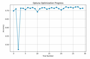
The following code plots the accuracy of each trial, producing a figure like the one below.
import matplotlib.pyplot as plt
import pandas as pd

df = study.trials_dataframe()

plt.figure(figsize=(8, 5))
plt.plot(df["number"], df["value"], marker="o", linestyle="-")
plt.xlabel("Trial Number")
plt.ylabel("Accuracy")
plt.title("Optuna Optimization Progress")
plt.grid()
plt.show()
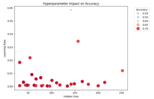
We can also visualize the relationship between hyperparameters and accuracy using a scatter plot. The optimal hyperparameters are located toward the lower-left area. Note that this 2D plot does not include information about the batch size.
import seaborn as sns
import matplotlib.pyplot as plt

plt.figure(figsize=(8, 6))
scatter = sns.scatterplot(x=df["params_hidden_size"], y=df["params_lr"], size=df["value"], hue=df["value"], palette="coolwarm", sizes=(20, 200))

plt.legend(title="Accuracy", bbox_to_anchor=(1.05, 1), loc="upper left")

plt.xlabel("Hidden Size")
plt.ylabel("Learning Rate")
plt.title("Hyperparameter Impact on Accuracy")
plt.show()
5. Conclusion
Using Optuna, we were able to easily perform hyperparameter optimization based on Bayesian optimization. In this example, we used a neural network with a single hidden layer, but further improvements such as increasing the number of hidden layers could enhance accuracy.